Modeling Production Lines and Basic Factory Dynamics

This demonstration is intended to introduce the concepts related to Little's law, starting first with a balanced line and validating the relationship, then moving to an unbalanced line, then adding uncertainty. The Penny Fab is a tandem production line, one where the four processing steps are organized serially.

Additionally, this demonstration will construct the production line simulation models in a couple of steps:

Baseline Balanced Deterministic Model: serial set of servers
Unbalanced Deterministic Model: requires the addition of queues in between the servers to buffer out uneven processing rates.
Stochastic Processing Times: requires the addition of random number generators for generating processing times from a distribution
An Arrival Process: rather than recirculating the entities in the system, an open system requires an arrival generator
Encapsulate Workstations: Encapsulate the ProcessTime, Queue, and Server into a single Workstation block. This encapsulation process makes it easy to manipulate the workstation as one object, and replace the workstation block with one that exhibits a different behavior,

Penny Fab and Basic Factory Dynamics
Balanced Production Line
Unbalanced Line
Worst Case Performance
Practical Worst Case Performance
Basic Factory Dynamics
Arrival Process
Encapsulated Workstation Blocks

Penny Fab and Basic Factory Dynamics

We're interested in examing the relationship between:

The bottleneck rate (): the production rate of the workstation having the highest long-term utilization
The raw process time (): the sum of the long-term average process times of each workstation in the line, or the amount of time it would take one job to traverse an empty line
The critical WIP (): the WIP level for which the line achieves its maximum throughput () with minimum cycle time ().

We seek to show: $W_0=r_b T_0$

Balanced Production Line

In this example, each machine takes exactly 2 hours to perform its operation. Since the capacity of each machine is the same and equals one penny every 2 hours, any of the four machines is the bottleneck. Therefore, $r_b=0.5$ penny per hour This production line is balanced since all stations have equal capacity. The raw processing time is simply the sum of the processing times at the four stations: $T_0=8$ hours and $W_0=r_b T_0=0.5\times8=4$ pennies

These results can be validated using the Simulation:

open('PennyFab_Deterministic')

setProcessNodeParameters('PennyFab_Deterministic', [1 1 1 1], [2 2 2 2]);
% Double Click on 'WIP_Queue' and $W_0$ should be set to 1;
set_param('PennyFab_Deterministic/WIP_Queue', 'NumberOfEventsPerPeriod', '1');
% Run the simulation.
simOut = sim('PennyFab_Deterministic', 'StopTime', '40');
% Examine each pop-up window.
Simulink.sdi.view

OUTPUT Analysis:

The throughput for each workstation, Figure 1, shows that one job comes through the workstation every 8 hours.
The throughput for the whole system, Figure 2, shows that one job comes through the system every 8 hours.
The cycle time for the whole system, Figure 3 show that the cycle time for each job that comes through the system is 8 hours.
Finally, the WIP for the whole system, Figure 4, shows that there are typically 0 jobs waiting in the queue. The jumps to 1 account for the job passing through the queue instantly before entering the system.

Exercise: Increment $W_0$ from 1:10. Run the system and describe the changes to the system. Discuss warm-up period.

Suppose now we want to be able to do analysis on the data rather than just looking at graphs:

 set_param('PennyFab_Deterministic/WIP_Queue', 'NumberOfEventsPerPeriod', num2str(4));
 simOut = sim('PennyFab_Deterministic', 'StopTime', '1000');
 getCycleTime(simOut)
 getThroughput(simOut)

ans =
     8

ans =
    0.5000

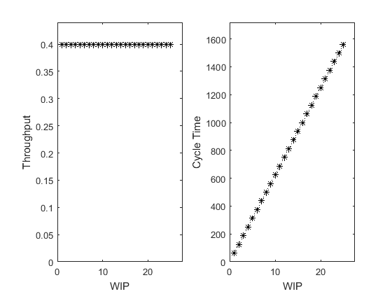
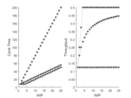
The function PennyFabScript_BestCasePerformance(ParallelMachineCount, ProcessingTime, varargin) simulates the Best Case Performance of a Tandem Production Line and sweeps over WIP levels from 1 to 25

SimWrapper_PennyFab_BestCasePerformance([1 1 1 1], [2 2 2 2], {'PlotsOn'});

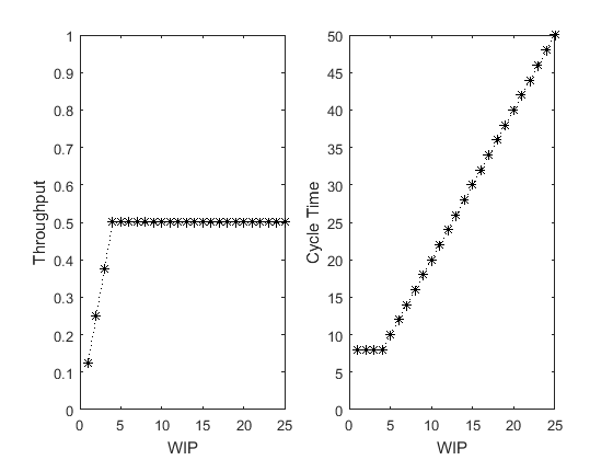
From a performance standpoint, it is clear that Penny Fab One runs best when there are four pennies in WIP. Only this WIP level results in minimum cycle time $T_0$ and maximum throughput $r_b$ – any less and we lose throughput with no decrease in cycle time; any more and we increase cycle time with no increase in throughput. This special WIP level is the critical WIP (W0) $W_0=r_b T_0$

These graphs and this formula reveal an interesting and fundamental retlationship between WIP, cycle time, and throughput; it is known as Little's Law. WIP = TH x CT Little's law holds for all production lines, not just those with zero variability (an exercise for later). However, it does not hold precisely for less-than-infinite times except under very special circumstances. Nonetheless, we will use it as a cnojecture about the nature of manufacutring systems and use it as an an approximation when it is not exact.

Unbalanced Line

Next we'll look at an unbalanced line.

The system paratmeters are set as follows (Table 7.1)

Station Number = [1 2 3 4]
Number of Machines = [1 2 6 2]
Process Time (hours) = [2 5 10 3]
Calculated Station Capacity = [0.5 0.4 0.6 0.67]

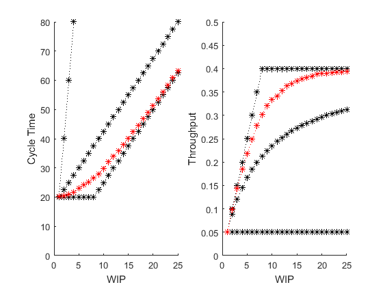
SimWrapper_PennyFab_BestCasePerformance([1 2 6 2], [2 5 10 3], {'PlotsOn'});

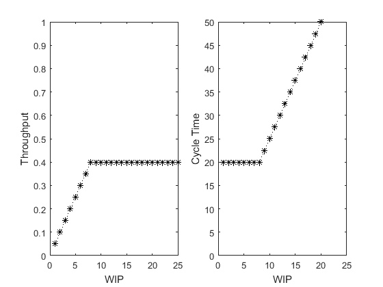
Does this agree with the relationship discussed above? Since the bottleneck station is station 2, $r_b=0.4$ penny per hour, and $T_0=2+5+10+3=20$ hours. $W_0= T_0 r_b=0.4x20=8$ pennies. This agrees with the graphs in the above figure.

Worst Case Performance

The system performance that has been explored so far is known as Best Case Performance which denotes the maximum throughput and minimum cycle time achievable for a given WIP level. However next we'll characterize, the worst case and practical worst case performance.

SimWrapper_PennyFab_WorstCasePerformance([1 1 1 1], [2 2 2 2], {'PlotsOn'});
SimWrapper_PennyFab_WorstCasePerformance([1 2 6 2], [2 5 10 3], {'PlotsOn'});

The worst case performance can result from batch moves.

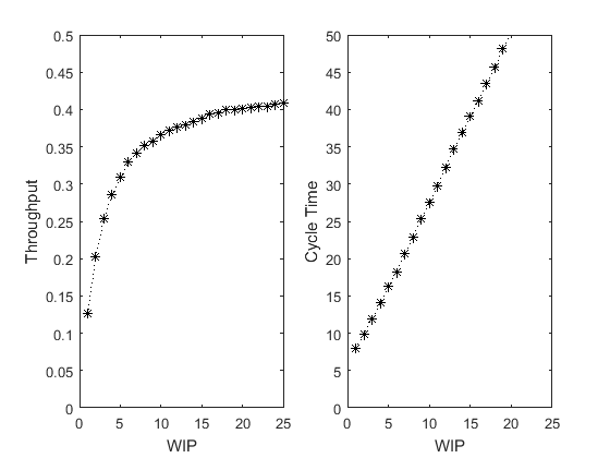
Practical Worst Case Performance

Both the best-case and worst-case performances occur in systems with no randomness. There is variability in the worst-case system, since jobs hav eidfferent process times; but there is no randomness, sincall prcoess times are completely predictable.

The practical worse case requires maximum randomness scenario:

The line must be balanced
All stations must consist of single machines
Proces times bust be random and occur accodring to the exponential distribution

In the simulation, queues have been added between each of the servers to buffer this randomness and prevent unnecessary blockage and starvation of the workstations.

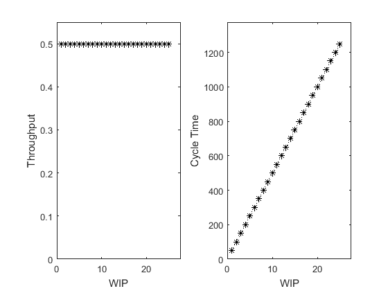
open('PennyFab_Stochastic')
SimWrapper_PennyFab_PracticalWorstCasePerformance([1 1 1 1], [2 2 2 2], {'PlotsOn'});
SimWrapper_PennyFab_PracticalWorstCasePerformance([1 2 6 2], [2 5 10 3], {'PlotsOn'});

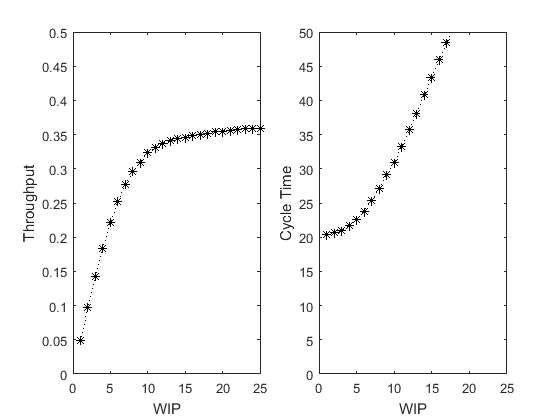
Basic Factory Dynamics

With the formulas validated we can put them together:

BasicFactoryDynamics([1 1 1 1], [2 2 2 2]);

Where does the unbalanced stochastic system performance fit into the basic factory dynamics?

FactoryDynamicsSol = BasicFactoryDynamics([1 2 6 2], [2 5 10 3], {'PlotsOff'});
PennyFabTwoSol = SimWrapper_PennyFab_PracticalWorstCasePerformance([1 2 6 2], [2 5 10 3], {'PlotsOff'});
    figure('Name','Basic Factory Dynamics')
    subplot(1,2,1)
    hold all
    plot(1:25, FactoryDynamicsSol (1:25,1,1), 'k*:')
    plot(1:25, FactoryDynamicsSol (1:25,1,2), 'k*:')
    plot(1:25, FactoryDynamicsSol (1:25,1,3), 'k*:')
	 plot(1:25, PennyFabTwoSol (1:25,2), 'r*:')
    axis([0 25 0 80])
    xlabel('WIP')
    ylabel('Cycle Time')
    hold off
    subplot(1,2,2)
    hold all
    plot(1:25, FactoryDynamicsSol (:,2,1), 'k*:')
    plot(1:25, FactoryDynamicsSol (:,2,2), 'k*:')
    plot(1:25, FactoryDynamicsSol (:,2,3), 'k*:')
plot(1:25, PennyFabTwoSol (1:25,3), 'r*:')
    axis([0 25 0 0.5])
    xlabel('WIP')
    ylabel('Throughput')
    hold off

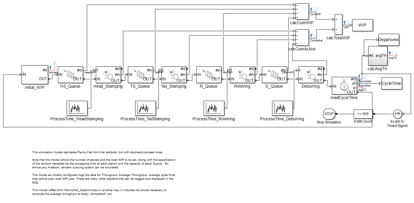
Arrival Process

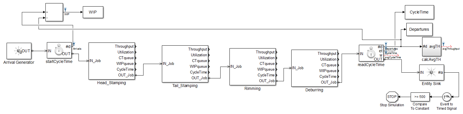
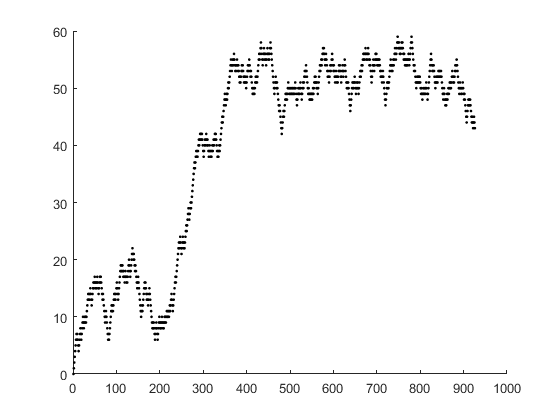
Up until this point, we have only considered closed systems with a constant WIP (CONWIP) level. But in practice, flow lines are subject to an arrival process. In this model, the production line is an open system subject to an external arrival process, the "Arrival Generator" block.

 open('PennyFab_ArrivalProcess')

setProcessNodeParameters('PennyFab_ArrivalProcess', [1 1 1 1], [2 2 2 2]);
% Set 'Arrival Generator' to an Exponential Distribution with mean 2
set_param('PennyFab_ArrivalProcess/Arrival Generator', 'Mean','2', 'Distribution', 'Exponential');
simOut = sim('PennyFab_ArrivalProcess', 'StopTime', '1000', 'SaveOutput', 'on');
WIP = simOut.get('WIP').signals.values;
figure
scatter(1:length(WIP), WIP, 'k.')

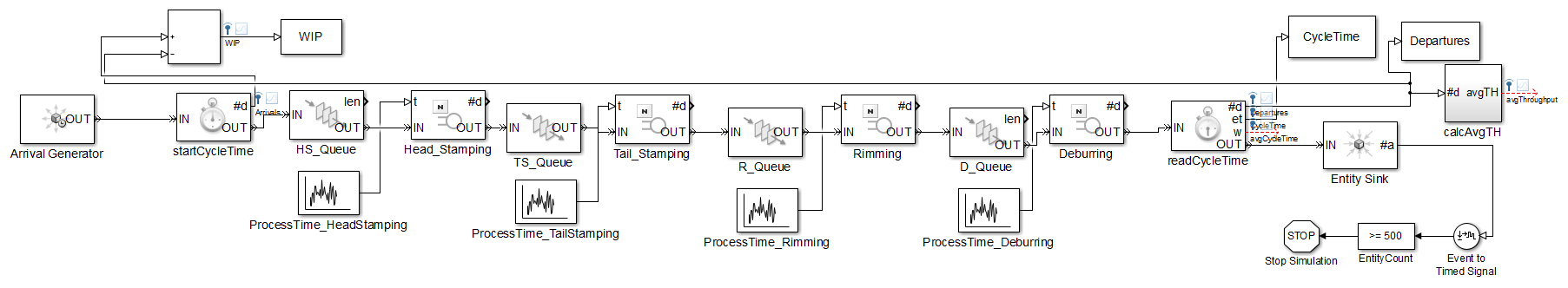
Encapsulated Workstation Blocks

One goal of this introductory section is to build up a production line model. In the balanced deterministic production line, the buffers (or queues) in between each stage are unnecessary and their capacity could be set to 0. However in the unbalanced production line, these queues are required to buffer out uneven production rates. Then in the stochastic production lines, the ProcessTime blocks are added to provide flexibility to set processing time distributions. Also, the queues are necessary to buffer out uncertainty in arrival and processing times. The last step of introducing the production line models is to encapsulate the ProcessTime, Queue, and Server into a single Workstation block. This encapsulation process makes it easy to manipulate the workstation as one object, and replace the workstation block with one that exhibits a different behavior, e.g. a workstation with failures, which will be an important feature for the next section.

open('ProdSys_PennyFab')
setProcessNodeParameters('ProdSys_PennyFab', [1 1 1 1], [2 2 2 2]);